Expressing Confidence in Models and Model Transformation

When modeling software for physical systems (such as robots, drones or industrial machinery), the models need to represent the reality as accurately as possible so that both the system representation, and more importantly, its simulations are trustable.

In this sense, an important fact to take into account is that these particular kind of systems as well as their interaction with their environment are subject to uncertainty. Thus, they must precisely consider that it affects their elements, the relationship between them and their behaviors.

The term uncertainty involves imperfect and/or unknown information. It appears every time we perform estimations, approximations, measurements or we face unknown properties of systems. While uncertainty is intrinsic in most engineering disciplines such as mechanical, electrical or aeronautical—and is explicitly taken it into account in models and model simulations—software engineers do not usually consider it when modeling software. For instance, well-known and widely used modeling notations and languages (such as UML) do not provide any support to express uncertainty.

We focus on two different types of uncertainty present in software models: measurement uncertainty (i.e., the inability to know with complete precision a value) and confidence (i.e., the degree of belief we have on the actual existence of model elements).

In this work, we propose how to quantitatively represent these two types of uncertainty in software models and how to propagate it through model transformations.

This work won the Best Foundation Paper Award of the ACM/IEEE 21th International Conference on Model Driven Engineering Languages and Systems 2018 (MODELS 2018). You can download our Expressing Confidence in Models and in Model Transformation Elements paper to learn more about our approach.

1 Introduction

Measurement uncertainty is an intrinsic property of any physical system. This uncertainty can be due to different causes, such as unreliable data sources and communication networks, tolerance in the measurement of the physical elements values, estimates due to the lack of accurate knowledge about certain parameters, or the inability to determine whether a particular event has actually happened or not. The explicit representation and proper management of measurement uncertainty is a crucial issue in any faithful model of a given physical system. This includes not only the (static) representation of the uncertainty, but also how it evolves and is propagated through the system operations.

In this paper, we focus on the treatment of a special kind of uncertainty, confidence, which refers to the quality of being certain about something, e.g., up to what extent something is true or will happen. In our context, we will assign confidence to model elements and model transformation rules.

The former kind of confidence refers to the degree of belief that we have on the actual existence of an entity, i.e., the real entity that the model element represents. A very typical example occurs in systems whose objects represent events from the physical environment, such as those produced by (unreliable) sensors that take measures, which can sometimes be false negatives—i.e., the event has occurred but it was lost, or the system did not record it properly. Similarly, if we consider robots or drones that move from one point to another and whose exact position always yields a margin of error of millimeters or even centimeters, the precise location of a moving artifact is also subject to uncertainty, and therefore we need to assign a level of confidence to it. Likewise, in a social network environment, the establishment of certain derived relationships between two objects (friendship, closeness, preference) may be subject to uncertainty because the person or program estimating such a derived relationship may not be fully reliable, or completely sure about his judgment—and therefore it may have some associated margin of error.

To assign confidence to model elements—both to objects and to relationships—we propose the use of attributes that permit estimating the confidence (i.e, the degree of belief) that we have on their existence, by means of probabilities associated to them.

Furthermore, model transformations (hereinafter, MT) may be subject to uncertainty, too, due to several factors. First, some transformation rules may have some associated uncertainty, when we do not have a 100% confidence on them—for example, a rule of a recommender system that generates a wouldLike relationship between a user and a product based on a set of preferences and a history of user actions may not be 100% accurate, and therefore we need to ‘qualify’ the results with this kind of information. Second, during the rule matching process, uncertainty may also be considered, due, for example, to the comparison of inaccurate attribute values, that yields an uncertain Boolean value [4]. Finally, the confidence and uncertainty of the input model elements must be propagated to the output elements, too, qualifying them accordingly.

In this paper we identify and classify some types of confidence that can occur both in the models and in the transformations among them, and we discuss how to incorporate them into the model elements and into the transformation rules, being able to quantitatively represent that confidence, and to propagate it through model transformations.

The article is organized in six sections. After this introduction, Section 2 briefly presents the background of our work. Then, Section 3 describes our proposal, and introduces an example that is used to motivate it, and to illustrate its main concepts and mechanisms. Section 4 describes some evaluation exercises we have conducted to assess the expressiveness and correctness of our proposal. Finally, Section 5 relates our work to other similar approaches and Section 6 concludes and outlines some future work.

2 Background

To set the paper terminology, this section briefly describes the context of the work and the main concepts used in the paper.

2.1  Models and Model Transformations

Here we will use the standard notions of models and model transformations (MT) used in MBSE [5]. A model is the representation or specification of some system, component or application, from a given point of view, and with a particular purpose. Models are represented as graphs whose vertices and edges are typed, and may have typed attributes. A models conforms to a metamodel, which specifies the language in which a family of models is expressed, including the language concepts, the relationships and constraints among them, and the well-formed rules of the language. Metamodels are models, too.

A MT is the algorithmic specification (declarative or operational) of the relationship between models. In this paper, we will focus on rule-based MTs, which are those defined in terms of a set of rules that determine how a set of objects and relations in the source model (defined by means of a pattern) are transformed into another set of objects and relationships between them in the target model. The source and target model can coincide, like in the case of in-place model transformations [26].

In our context, it is important to note that most rule-based model transformation languages share a common structure in the definition of their rules:

• A Selection phase that identifies the source elements that will trigger the rule. They constitute the antecedents of the target elements produced by the rule.
• A Matching phase that checks whether the values of the attributes of the selected events meet the requirements and conditions of the rule, and calculates the values of the attributes of the elements generated by the rule (using Boolean comparison operators, and connectives between them).
• A Production phase that generates the target model elements, and the trace links, if appropriate.

2.2  Uncertainty

Uncertainty is the quality or state that involves imperfect and/or unknown information. It applies to predictions of future events, estimations, physical measurements, or unknown properties of a system [19]. For example, measurement uncertainty (MU) refers to the inability to know with complete precision the value of a quantity. Confidence (C) refers to the degree of belief that we have on the actual existence of an entity (in our case, a model element).

Both types of uncertainties can be represented in different forms, and using different formalisms. For example, measurement uncertainty can be expressed by means of a probability distribution associated to every uncertain variable, representing the distribution of the dispersion of its values. This is the approach used by, e.g., the UML Profile for MARTE [28]. However, this approach represents some limitations when calculating the aggregated MU of the result of an operation that involves operands with different probability distributions. A more widely adopted approach among engineers of different disciplines to represent MU, is defined by the GUM [20], which associates a standard uncertainty to any uncertain value, defined by the standard deviation of the measurements for such a value. Therefore, a Real number x becomes a pair (x,u), also noted x±u, that represents a random variable X whose average is x and its standard deviation is u. With this, if X follows a normal distribution N(x,u), we know that 68.3% of the values of X will be in the interval [x−u,x+u].

The GUM framework also identifies two ways of evaluating the uncertainty of a measurement, depending on whether the knowledge about the quantity X is inferred from repeated measured values (“Type A evaluation of uncertainty”), or scientific judgment or other information concerning the possible values of the quantity (“Type B evaluation of uncertainty”). In Type A evaluation of uncertainty, if X={x1, …, xn} is the set of measured values, then the estimated value x is taken as the mean of these values, and the associated uncertainty u as their experimental standard deviation  [19]. In Type B evaluation, uncertainty can also be characterized by standard deviations, evaluated from assumed probability distributions based on experience or other information. For example, if we know or assume that the values of X follow a normal distribution, N(x,σ), then we take u=σ. And if we can only assume a uniform or rectangular distribution of the possible values of X, then x is taken as the midpoint of the interval, x=(a+b)/2, and its associated variance as u^2=(b-a)^2/12).

Uncertainty can also apply to Boolean values. For example, in order to implement equality and comparison of numerical values with uncertainty, the traditional values of true and false returned by boolean operators are no longer enough. Comparisons now need to return numbers between 0 and 1 instead, representing the probabilities that one uncertain value is equal, less or greater than other. This leads to the definition of Uncertain Booleans, which are Boolean values accompanied by the level of confidence that we assign to them. Therefore, an UBoolean value is a pair (b,c) where b is true or false, and c∈[0,1] represents the confidence we have on such a value; of course, (b,c)=(≠b,1−c). UBoolean is a proper supertype of Boolean and its associated operations [4]. Note that this approach should not be confused with fuzzy logic: although both probability and fuzzy logic represent degrees of subjective belief, fuzzy set theory uses the concept of fuzzy set membership, i.e., how much an observation belongs to a vaguely defined set, whilst probability theory uses the concept of subjective probability, i.e., the likelihood of an event or condition [22].

This is why we will also use probability theory to express Confidence, assigning probabilities to model elements. The confidence that we assign to a model element represents the degree of trust that we have on their actual existence. Here it is interesting to distinguish between the real and the model elements: the former ones happen in reality; the latter are the ones contained the system model, representing the real ones. It may be the case that the real object exists in reality but the system model has not captured it (i.e., a false negative), or that the model transformation rules generate an object or relation that does not actually exist (i.e., a false positive). The first case can be due to unreliable sources (e.g., defective sensors), while the second case is normally due to unreliable beliefs on the transformation patterns and rules.

With all this, there are different kinds of uncertainty that we need to consider in this work for model elements.

• Uncertain elements in the source models (for example, missing objects or relations in reality, despite the fact that they actually exist in the model), or elements in the target model that were wrongly generated.
• Lack of precision (i.e., measurement uncertainty) in the values of the attributes of the source model elements, due to the imprecision of the measuring methods or tools.
• Lack of precision in the decisions/matches due to the uncertainty of comparison operators (=, <, >, …) between uncertain values of attributes. For example, when comparing two real values with uncertainty, such as a=2.0±0.3 and b=2.5±0.25, we obtain that a<b with a confidence of 0.893 [4]. Any decision that we take based on such a comparison should then be subject to uncertainty.
• Lack of precision due to uncertainty of logical composition operators (or, and, not) between uncertain statements.
• Lack of precision in the values of the attributes of generated elements, due to the propagation of uncertainty in their computation from the elements’ attributes.
• Lack of precision in the MT rules, due to incomplete or erroneous assumptions about the environment in which the system operates, or unreliable beliefs, which may influence the confidence of the MT rule.

For dealing with uncertainty we have used the U-Model conceptual model defined in [34] as a reference framework, trying to be aligned with it. When it comes to concrete concepts that specialize some of the high-level U-Model concepts, such as measurement uncertainty, or confidence, we will use standard references. In particular, we will use the VIM [21] and the GUM [19] for all measurement uncertainty related matters, and probability theory [17] for dealing with confidence.

3 CONFIDENCE IN MODELS AND MT RULES

3.1 Expressing confidence in model elements

As previously mentioned, we are interested in assigning probabilities to model elements. These probabilities represent the confidence we have on their occurrence.

To represent the confidence of a model element we will make use of a new abstract class called ProbableElement, from which all the uncertain elements of the model would inherit. This class has an attribute (confidence, a Real number between 0 and 1) that indicates the confidence assigned to the existence of the element, expressed as a probability.

For example, if an object is derived from a rule that has a confidence of 99%, a first approach could be to assign a probability of 0.99 to that object; or if the object represents a system event, for which we know that the probability of obtaining a false positive is F = 0.001 (due to the accuracy of the sensor that generates it), we could assign to the object a probability of 1 − F = 0.999.

Note that this new class would play a similar role to the one played by class NamedElement in the UML metamodel. In addition, if an item does not inherit from that class, its confidence is 1.

Although not only object instances but any other model element (association, transition, etc.) can be assigned a confidence, in order to assign attributes to elements we will simply convert them into objects. For example, if we want to assign a probability to an Association, we can convert it into an Association Class, or just into a Class with the appropriate references to the two related classes. Therefore, in following we will focus on objects only.

3.2 Expressing confidence in MT rules

As mentioned above, most rule-based model transformation languages share a common structure in the definition of their rules. Depending on the rule phase, different kinds of uncertainties need to be considered in order to assign a confidence to the generated target elements.

• The Selection phase identifies the occurrence of the elements that trigger the These objects constitute the antecedents of the elements produced by the rule. Thus, in this phase, the confidence of the antecedents must be considered, that is, the probability of occurrence of the elements that trigger the rule.
• The Matching phase checks whether the values of the attributes of the selected events meet the requirements and conditions of the rule, and calculates the values of the attributes of the elements generated by the rule. In this phase we need to consider the uncertainty that occurs in the comparison operations between uncertain values, and the combination of these comparisons using logical connectors (or, and, etc.). The measurement uncertainty that occurs when calculating the values of the attributes of the generated elements should also be considered in this phase, propagating the corresponding measurement uncertainty of the operands.
• The Production phase generates the elements of the output In this phase we need to take into account the

confidence of the rule itself, represented by a probability that captures the possible imprecision of the rule due to incomplete or possibly erroneous assumptions caused by the environment in which the system operates, or other factors that influence the confidence in the rule. This rule confidence can be calculated by Bayesian networks, as proposed by Cugola et al. in [12] for CEP systems, by expert knowledge, or by any other means. For example, in a system that models a social network, a rule can trigger the creation of a relationship of friendship between two users, and we know that the confidence that we have on such a derivation rule is 89%. Therefore, we will assign a confidence of 0.89 to the MT rule. Note that confidence in a MT rule is not the same as the probability that the rule will be triggered, which is what other authors use when simulating rule-based systems [3].

In summary, our approach assumes that the confidence of an object generated by a MT rule depends on three main issues: (a) the confidence level that we have on the occurrence of the source objects of the rule (antecedents); (b) the confidence level that we have on the matching and comparison operations performed by the rule to trigger the production of the target objects, as well as the computation of their attributes; (c) and, finally, on the confidence that we have on the rule itself.

This means that, given a rule R whose antecedents are objects o1, …, on , that performs a matching process mR and produces a target object o, the probability of o is given by the formula (1):

P (o) = P (o1, …, on ) · P (mR ) · P (R)

where: P (o1, …, on ) is the combined probability of the antecedent objects—for example, in case they are all independent, P (o1, …, on ) = P (o1) · … · P (on ), otherwise conditional probabilities should be used, as detailed in, e.g., [36]; P (mR ) is the confidence level of the matching process, based on the uncertainty due to comparison operations (=, <, …) between uncertain values, and logical operations between uncertain booleans (and, or, …); and P (R) is the rule confidence—which, as stated above, can be calculated by Bayesian Networks, by expert knowledge, or by any other means; in this paper we are not concerned on how such a probability is computed, but on how it is represented and taken into account.

In case a rule produces a set of elements, the formula above will be used for each generated element.

3.3 A motivating example

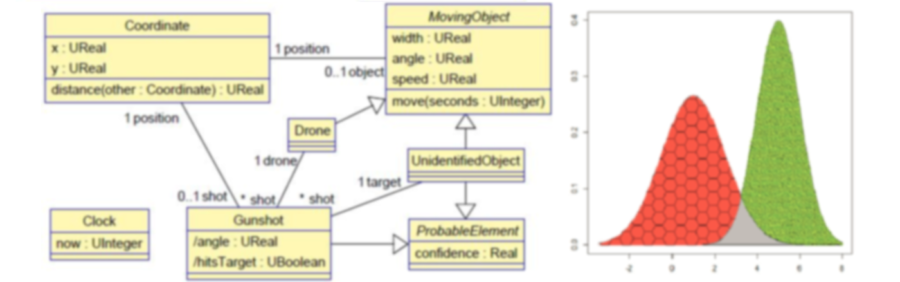
To illustrate our approach let us assume a system whose elements are described by the metamodel shown below. Surveillance drones are in charge of ensuring that no unidentified object gets close to the area they protect. For simplicity, we assume that all objects move in a planar surface (and thus their position is given by a pair of coordinates x and y); in the direction dictated by their angle attribute (expressed in radians), and with a given speed (in m/s). The size of a moving object is determined by its diameter (attribute width, also in meters). Movements are performed by operation move which updates the coordinates of the object based on its current angle and speed, and the number of elapsed seconds since the last movement. Times are expressed using the POSIX time convention, i.e., by the number of seconds since January 1, 1970 [22].

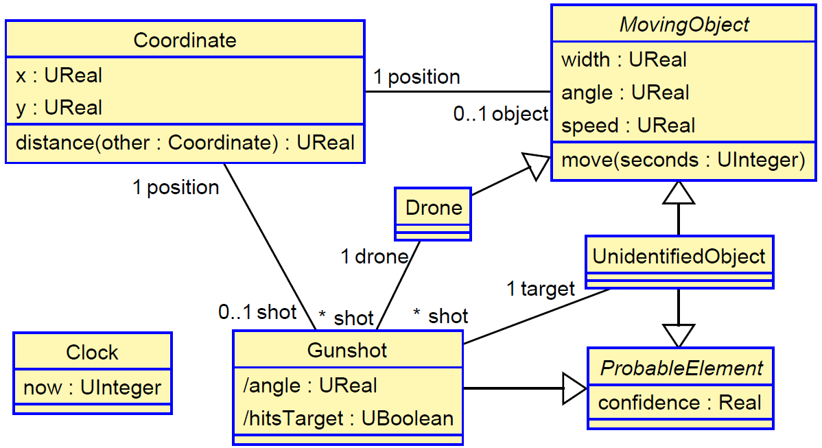
If a drone detects that an unidentified object is moving at a speed higher than 30 m/s and gets closer than 1000 m to its position, the drone identifies it as a threat, and shoots at it. The potential shot is represented by an object of class Gunshot. The position of the Gunshot object coincides with the position of the drone that shoots at the target, and its attributes are calculated as shown in the excerpt of code below. Attribute hitsTarget is an uncertain boolean because of the measurement uncertainty of the variables, and the tolerance of the shooting instruments.

Note the use of variables of types UReal and UBoolean in this code, which represent uncertain reals and booleans, respectively [6]. As previously mentioned, when dealing with real-world entities, models need to take into account the inability to know, estimate or measure with complete precision the value of the represented quantities. This is why, in general, a measurement result that determines the value of a quantity “is only complete when it is accompanied by a statement of the associated uncertainty” [23, 24].

Objects of classes UnidentifiedObject and Gunshot have an associated confidence, representing the fact that the domain rules that detect a moving object and identify that it is a threat, are subject to some degree of uncertainty. Such confidence is then translated into the confidence of the derived rule that decides whether to shoot or not at the target. We assume a precision of ±1 second in all time measurements, and this is why attribute now of object Clock is of type UInteger [6].

The system contains at that moment two drones (d1, d2) and three unidentified objects (o1, o2, o3). These three objects have an associated confidence due to possible errors in the radar that detects moving objects (normally, the confidence of a sensed or detected object coincides with 1 − F , where F is the probability of a false positive of the object occurrence).

The behavior of the system can be represented by means of an in-place model transformation that determines how the state of the system evolves with time. In our case, we will suppose a discrete simulation of the system whereby a MT will calculate the state of the system every second, based on the previous state.

Then, given a model that represents the state of the system at a given moment in time, a MT will perform the following actions.

• For every UnidentifiedObject (with a confidence greater than 0.65) moving at a speed higher than 30 m/s, which has not already been shot (with a confidence of hitting the target higher than 0.95), and with a drone less than 1000 m away from it, a GunShot object (that relates the drone with the target) will be
• The coordinates of all moving objects will be updated, using their move() In this case, the value of the argument is 1, assuming that the MT simulates the behavior of the system every second.

Finally, attribute now of object Clock will also be updated, reflecting the passage of that time.

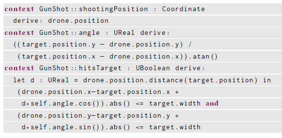
For example, the in-place ATL transformation below could implement such behavior.

Let us explain how the confidence of the newly created objects is calculated. In this case the confidence is computed in rule shoot when creating the Gunshot object (lines 19–23), and in rule moveUnidentifiedObject when re-calculating the confidence attribute of the object (line 48). In this second case, we assume that the confidence of the object does not change when it moves. In the former case, to compute the confidence of the GunShot object in the shoot rule we make use of formula (1) above.

The expression of the confidence of the gs object depends on the confidence of the antecedents (line 19): the unidentified object u and the drone d. The first one is given by u.confidence and the second one is 1.0 because drones are certain objects.

The second operand of formula (1) is the confidence of the matching operations used in the rule. To compute it we simply make use of method uncertainty() of type UBoolean, which returns the confidence of the uncertain boolean—i.e., the second component of the pair (b, c). We can see (line 22) how it is applied to the filter expression used in the left-hand side of the rule, and it captures the accumulated probability of all comparison operations between uncertain reals, and its composition through logical connectors. The way in which such an operation works is detailed in [6]. Basically, it combines the probability of the operands using the composition laws of the logical operations. In this case we are assuming all operands are independent, and therefore logical conjunctions result in probability multiplications.

Finally, we have assumed that the confidence of rule shoot, that generates the shots, is shootC = 0.99 (line 23), due to the possible inaccuracies in the estimation of the decision parameters. The other rules are always accurate.

With this, the object diagram that represent the system at time 1524199496 (i.e., after 1 second) is shown below.

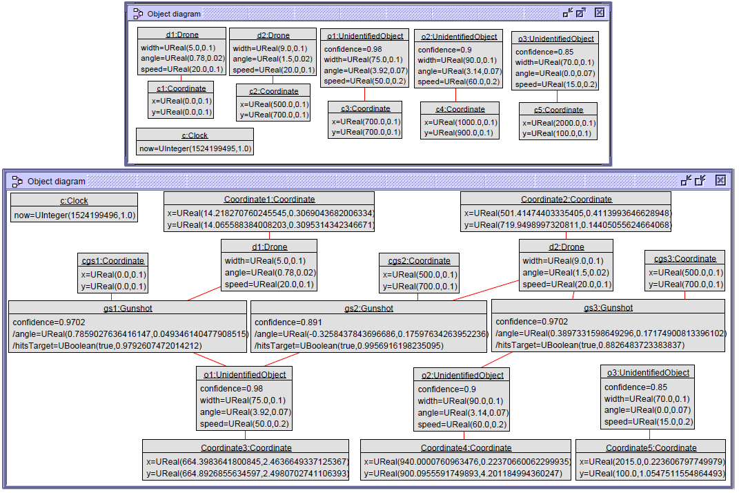
We can see that the clock has elapsed 1 second, that all drone and unidentified objects have moved (hence their coordinates have been updated), and that the two drones have shot at their targets. Drone d1 has shot at object o1 with a confidence of 0.9702, and with a likelihood of hitting it of 0.97926. Drone d2 has fired two shots. The first one at object o1 with a confidence of 0.891 and the second one at object o2 with a confidence of 0.9702. The chances of hitting these targets are 0.99569 and 0.88264, respectively.

Note how the non-recursive semantics of the ATL refining mode work in this case [35]: all rules check the matches first, and then create the target objects in a second step. This is why object o1 is shot twice, even when the two gunshots have probabilities of hitting the target higher than 0.65. Should we have used another in-place transformation language with recursive semantics, e.g. Henshin [5] or any other graph transformation language that modify the target model after the application of each individual rule, only one shot at object o1 would have been fired.

Note as well that the ATL code shown above in Listing 2 is just a sample of how it should work. Unfortunately, the extended type system that permits dealing with UReal and UBoolean values and their operations are not currently implemented in ATL. This is why we have used LinTra [9] to develop the implementation of all our model transformations, as discussed below.

4  Evaluation

4.1  Case studies

In order to evaluate the expressiveness and applicability of our proposal, we have also modeled two further case studies, from separate domains in which our approach can be effectively used (apart from the motivating example in Section 3, which was in the cyber-physical systems domain): predictive models and run-time models. The implementation of this two case studies, as well as the one presented in Section 3, are available from our group’s website [1], Git repository [2] and ReMoDD repository [6].

A social media recommendation system

The following is an example of a predictive model. It is a reduced version of a recommender system in a social media environment, whose metamodel is shown below. At the basic level there are Users and Items. Users follow other users, and like items. Items can be pictures, tweets, or products from a catalog. We are interested in modeling a system whose behavior, in addition to representing these elements and their relations, is also able to infer further relationships. For the sake of simplicity, we have omitted many details from the real system, such as user circles, item tags, and further relations between the objects such as retweets.

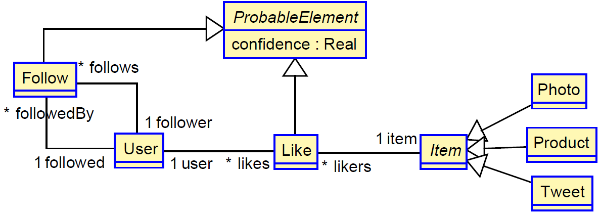
For example, a business rule can estimate that if more than 200 followers of a user like an item, it is quite likely that the user likes it too. Similarly, if user A likes more than two thirds of the likings of user B, it may be the case that A could be interested in following B, too.

Our approach permits expressing these issues in a very natural way. We have reified the relations Like and Follow to be able to assign confidence to them, making them regular classes (another option would have been to make them association classes). Links defined by users have a confidence of 1.0. Links derived by the system will have a smaller confidence. Then the user could accept them (modifying its confidence to 1.0) or reject them (making it 0.0 or simply removing the derived link from the model).

A model transformation can be in charge of recalculating all relationships and their confidence after a user manually creates or removes a relationship, or accepts or rejects one suggested by the system. The code below shows part of the behavior of such a model transformation, namely the rule that suggests a Like relationship between a user and an item (once again, we are presenting it here in ATL, for understandability purposes).

The rule counts those users who are related to a given user u through a Follow relationship with a confidence higher than 0.95 (line 9) and, from those, the rule selects those who like the item with a confidence higher than 0.85 (line 11). Then, the rule checks whether the number of such followers is higher than 500 (line 12) and there is no previous Like relationship between the user and the item (line 13). If so, it creates a Like object representing such a relationship.

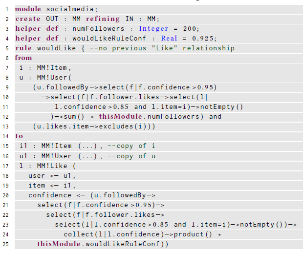
Given that users and items have no associated confidence (they are certain objects), the confidence of the newly created Like relationship only depends on the confidence of the Follow and Like relationships that the rule uses in the selection process (these are the antecedents in this case). Therefore, it is a matter of navigating the relations that are used (lines 20–24), and multiply their confidence (line 24). Given that we are not dealing in this example with measurement uncertainty of the attributes of the objects, there is no need to compute the uncertainty in the matching phase of the rule. Finally, we need to take into account the production phase of the rule, multiplying the result by the rule’s confidence (line 25), which in this case we assume it is 0.925 (line 4).

Modeling confidence in run-time models

To illustrate our proposal in the case of run-time models we will use an example taken from the Complex Event Processing (CEP) domain. CEP [14, 24] is a form of Information Processing [8] whose goal is the definition and detection of situations of interest, from the analysis of low-level event notifications [10], also called simple events. Then, complex events are those that summarize, represent, or denote a set of other events. Complex events are derived by rules that define the relevant patterns of (simple or other complex) events, their contents, and their temporal relations. In fact, CEP can be considered as a special kind of streaming model transformations [7, 11], able to manipulate models whose elements are continuously produced or modified in high volume and with rapid rate of change.

In this context, let us suppose that we have a smart house, with sensors that permit detecting three basic parameters: temperature, carbon monoxide (CO) level, and whether the main door is open or not. These values are periodically sensed and notified by means of Home events, which also include information about the house id, the time at which the event was issued, the coordinates of the house, and its size in square meters. We also want to monitor whether the people living at a house are inside or not. Therefore, we suppose that they periodically issue Person events with their location (coordinates x and y).

The figure below shows the metamodel of such a system. Classes Person and Home represent the CEP simple events described above. Classes shaded with darker background color represent the complex events defined by the application:

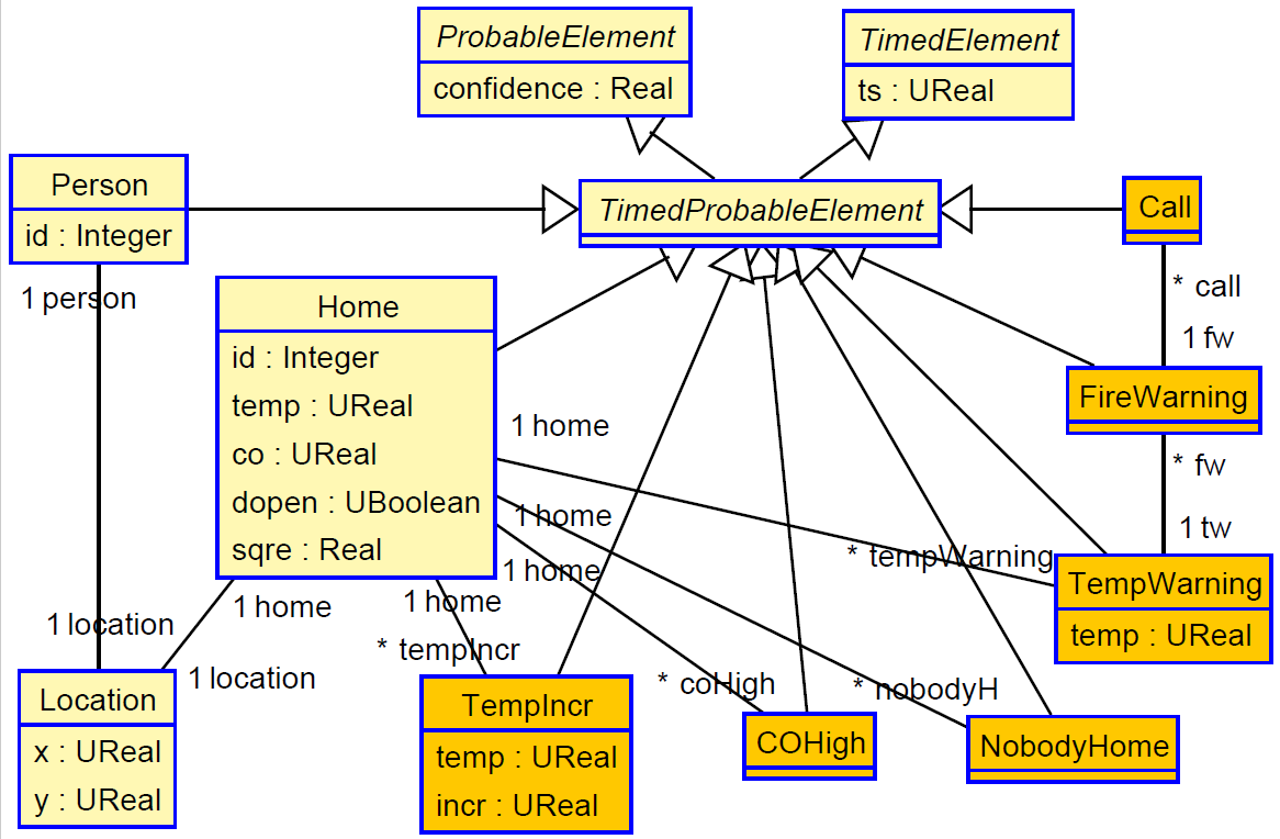
TempIncr: The temperature of the house has increased 2 or more degrees in less than one minute.

• TempWarning: Four TempIncr events are detected in less than 5 minutes, while temperature remains above 33 degrees.
• COHigh: CO levels exceed 5000 units.
• FireWarning: A COHigh event is detected, followed by a TempWarning event, everything within less than 5 seconds.
• NobodyHome: The main door of the house is closed and there is no person within the perimeter of the house.
• Call: A FireWarning event occurs after a NobodyHome event is detected; the fire department should be called.

Starting from the simple events, they are enriched with the measurement uncertainty of their attributes, and with the confidence we have on the event. For simple events, their confidence is given by (1−F(e)), where F(e) is the probability of a false positive for that event.

The confidence of the complex events is calculated by the following formula, as the product of three factors: (a) the confidence of its antecedents, (b) the confidence of the matching and comparison operations, and (c) the confidence of the rule itself. For example, the probability of the previous TempIncr event, created by the rule with the same name, is given by:

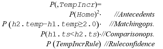
The code below shows a piece the ATL transformation that implements the rule that generates the TempIncr objects.

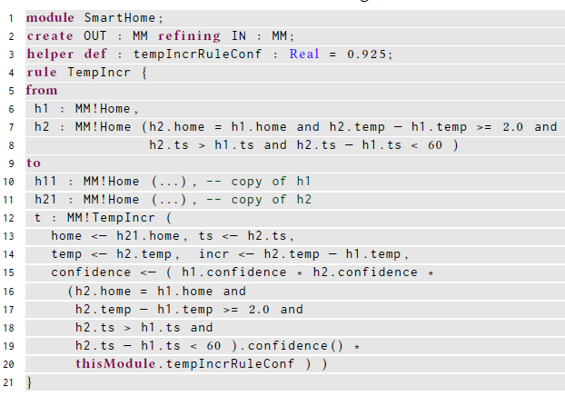
We can see how the rule computes all attributes of the complex event, including attribute confidence with the associated confidence, using the formula above.

Similar rules are in charge of generating the rest of the complex events. In addition, there is a dedicated rule that feeds in the model the objects that represent the basic events newly arrived, while another rule removes obsolete events, i.e., those objects whose timestamp falls outside the event window—hence simulating a streaming transformation.

This example also illustrates the need to consider confidence in CEP systems, something we also discussed in [27]. Instead of all events being equally probable, assigning confidence to events introduces an implicit prioritization mechanism, very useful for instance when two or more critical events occur (e.g., two Calls to the Fire Department). In these cases we could discriminate among them based on their probability, attending those most probable first.

4.2  Performance

In order to check the performance penalty introduced by our extension with uncertain types and its operations, we have created a set of synthetic models for our three case studies. For each case study, we present the number of elements in the model before and after the execution of the transformation, as well as the execution time of the transformation with and without uncertain types.

We have executed the experiments using Java 8 on a machine whose operating system is Windows 10 64-bits with 8 Gb of RAM and an Intel i7 processor with 8 cores of 1.6 GHz each.

Table 1 shows the performance of the Surveillance case study, for models of increasing sizes (from 101 to 100,001, being the single object the system Clock). In this case the overhead introduced by the uncertain types and most importantly by operating with them remains between 1.5 and 2.6. We can also see how the time taken by the MT exponentially increases with the size of the model (note that this is not due to our extension, but the nature of the MT itself).

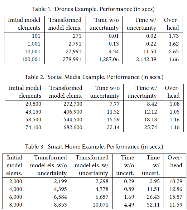
Table 2 shows the corresponding performance figures for the social media example. In this case the overhead is very small (between 0.05 and 0.16) because there are no attributes with measurement uncertainty. Therefore, calculations on attributes and logical comparison operations do not need to propagate such kind of uncertainty—even when the size of the transformed models is much bigger than the size of the source models.

Table 3 shows the opposite situation. In this case the number of created objects is smaller (merely a 10%), but the system needs to perform many operations on uncertain values (values of attributes and comparison operations between them). We can see how the model transformed taking into account the uncertainty introduces many new objects, which represent the relationships suggested by the recommendation rules. The overhead in this case is between 10 and 15 times, due to the need to operate with measurement uncertainty and to propagate it.

4.3  Discussion

Once we are able to assign confidence to model elements and to model transformation rules, this subsection discusses some aspects of our proposal, as well as some of its main benefits and limitations.

First, using our approach we could make decisions based on the confidence of the generated objects, before triggering the rules. For example, we could avoid shooting at the target if the confidence of the gunshot that is going to be generated is below a given threshold (0.3 for instance). Or we could discriminate between two calls to the fire department, attending the most probable one in case we do not have enough resources. Concerning the way in which we have added the information about the confidence to the model elements, we decided to make use of an abstract class (ProbableElement). This approach has both benefits and limitations. On the one hand, it is very natural and easy to use, and the confidence becomes a regular attribute of the model elements we are interested in. On the other hand, this mechanism is rather intrusive and not always possible to use—for instance, when dealing with legacy models for which the (un)certainty of their elements is unknown. An alternative solution could be the use of annotations, either internally in the model or externally by means of UML profiles or similar mechanisms. However, these annotations could greatly hinder the easy treatment and computations of the confidence attribute in all expressions.

Finally, the performance issue needs to be discussed. We have seen that in some cases, the fact of dealing with the calculation of the measurement uncertainty of the attributes, and its propagation through the operations and comparison operators, may introduce a significant overhead. This performance penalty has to be taken into consideration in the case of applications with very stringent response time requirements.

5  Related Work

In [33] the authors propose a conceptual model, called Uncertum, which is supported by a UML profile (UUP, the UML Uncertainty Profile) that enables including uncertainty in test models. Uncertum is based on the U-Model [34], extending it for testing purposes. UUP is a very complete profile that covers all different kinds of uncertainties. In particular, it defines three different measure packages (Probability, Ambiguity, and Vagueness) to facilitate annotating modeling elements with different uncertainty information and measures. Our work differs from it mainly in two aspects. On the one hand, we just cover one way of modeling confidence, using probability theory, while UUP also offers the use of possibility theory (ambiguity) and fuzzy sets (vagueness). On the other hand, our focus is slightly different. UUP was defined mainly for test modeling, i.e., creating test ready models that can be used to generate executable test cases, and therefore such type of modeling is less detailed than, e.g., modeling for automated code or for transforming the models, as in our case. This is mainly because, during test modeling, the work [33] is mainly interested in modeling test interfaces (e.g., APIs to send a stimulus to the system, and capturing state variables) and in the expected behavior of a system, and thus the importance lies on the expressiveness on the annotations on the model elements. However, we are interested in both representing that information and operating with it—for instance, to calculate derived values or to automatically compute the confidence of a target element generated by a model transformation rule. For semantic coherence, we decided to restrict our choices and use just probability theory to represent confidence levels, using one uniform approach, in this case probability theory. Otherwise, combining the uncertainty information expressed using different approaches would not make sense. For example, consider aggregating the uncertainty of two attributes of the same kind, one expressed using classical probabilities, and other using either vagueness (fuzzy logic), or ambiguity (e.g., Hartley or Shannon possibilistic measures of uncertainty).

This proposal is also inspired by existing works in the field of complex event processing (CEP), which can be considered a particular case of model transformations [11]. The work [3] offers a very interesting summary on the proposals to address the uncertainty in CEP systems, and that partially cover some of the ideas we have mentioned here. Among them, Wang [31] addresses the uncertainty in the selection phase, while Wasserkrug [32] and Cugola [9] deal with the other two phases using Bayesian Networks—each one using a different approach. In [27] we made a proposal covering the three phases in the case of CEP systems, using the extended type system for dealing with measurement uncertainty in UML and OCL defined in [4]. This greatly simplifies the representation of the uncertainty and its propagation, as we have seen in Section 3. In this paper we propose an extension of this proposal to the domain of the models and the transformations between them, generalizing significantly the results obtained, as well as their applicability.

There are various modeling works that deal with uncertainty, but they usually focus on aspects of uncertainty different from the ones we have described here. For instance, on the uncertainty on the models themselves and on the best models to use depending on the system properties that we want to capture [23]. Other works deal with the uncertainty of the design decisions, of the modeling process, or of the domain being modeled [18, 15, 13, 29, 12]. Our work differs from them since we are just concerned with the confidence we assign to the model objects, which is a different problem. We are not aware of other works that deal with uncertainty in model transformations, apart from the existing works on CEP systems mentioned above. In [16] the authors deal with the transformation of may-models [15], which are models subject to design uncertainties, but the transformations themselves are not subject to uncertainty. Moreover, the propagation of design uncertainty, due to its particular nature, is completely different from that of measurement uncertainty or of confidence in the model elements.

Other authors have also identified the need of counting on mechanisms to represent and manipulate physical values in software models [30], in particular units or real-time properties [25, 4]. Again this kind of uncertainty is different from the one treated here, although we have needed it in order to define the confidence of the model objects.

Finally, there is an active research area on probabilistic programming languages[1]. These programs are targeted to describe probabilistic models and then perform inference in those models. Our proposal here uses a simpler approach, assigning just probabilities to objects representing the belief that we have on their occurrence, which is the main focus of our work.

6  Conclusions

This contribution proposes the representation and management of the information about the confidence we have in the elements of the models, and how such confidence is propagated through model transformations. We have identified different types of uncertainty that can affect such confidence, and proposed a way to calculate the confidence of the elements generated by a transformation.

Our work can be continued in various directions. First, more and larger case studies should give us more feedback on the features and scalability of our approach. One particular aspect of interest is the application of our proposal to existing models and model transformations in the least intrusive way possible. In this respect, the use of high-order transformations could provide the required mechanisms to adapt existing MTs, adding confidence to their elements and rules. Finally, we are also working on the integrated support of all these mechanisms and tools within widely used model transformation languages, such as ATL.

 

REFERENCES

1. 1. Atenea research group’s official website, 2018. http://atenea.lcc.uma.es/projects/ConfidenceMandMT.html. Accessed: July
   2. LinTra Git repository, 2018. https://github.com/atenearesearchgroup/lintra.git. Accessed: July
   3. Agha, J. Meseguer, and K. Sen. Pmaude: Rewrite-based specification language for probabilistic object systems. ENTCS, 153(2):213–239, 2006.
   4. Alevizos, A. Skarlatidis, A. Artikis, and G. Paliouras. Complex event processing under uncertainty: A short survey. In Proc. of EDBT/ICDT’15, pages 97–103. CEUR-WS.org, 2015.
   5. Arendt, E. Biermann, S. Jurack, C. Krause, and G. Taentzer. Henshin: Advanced concepts and tools for in-place EMF model transformations. In Proc. of MODELS’10, volume 6394 of LNCS, pages 121–135. Springer, 2010.
   6. F. Bertoa, N. Moreno, G. Barquero, L. Burgueño, J. Troya, and A. Vallecillo. Expressing Measurement Uncertainty in OCL/UML Datatypes. In Proc. of ECMFA’18, number 10890 in LNCS, pages 46–62. Springer, July 2018.
   7. Bézivin. On the unification power of models. Journal on Software and Systems Modeling, 4(2):171–188, 2005.
   8. Burgueño, M. F. Bertoa, N. Moreno, and A. Vallecillo. Expressing confidence in model and model transformation elements, 2018. http://remodd.org/node/581. Accessed: July 2018.
   9. Burgueño, M. Wimmer, and A. Vallecillo. A Linda-based platform for the parallel execution of out-place model transformations. Information & Software Technology, 79:17–35, 2016.
   10. S. Cuadrado and J. de Lara. Streaming model transformations: Scenarios, challenges and initial solutions. In Proc. of ICMT’13, volume 7909 of
   11. LNCS, pages 1–16. Springer, 2013.
   12. Cugola and A. Margara. Processing flows of information: From data stream to complex event processing. ACM Comput. Surv., 44(3):15:1–15:62, 2012.
   13. Cugola, A. Margara, M. Matteucci, and G. Tamburrelli. Introducing uncertainty in complex event processing: model, implementation, and validation. Computing, 97(2):103–144, 2015.
   14. Cugola, A. Margara, M. Pezzè, and M. Pradella. Efficient analysis of event processing applications. In Proc. of DEBS’15, pages 10–21. ACM, 2015.
   15. Dávid, I. Ráth, and D. Varró. Foundations for streaming model transformations by complex event processing. Software and System Modeling, 17(1):135–162, 2018.
   16. Eramo, A. Pierantonio, and G. Rosa. Managing uncertainty in bidirectional model transformations. In Proc. of SLE’15, pages 49–58. ACM, 2015.
   17. Esfahani and S. Malek. Uncertainty in self-adaptive software systems. In Software Engineering for Self-Adaptive Systems II, number 7475 in LNCS, pages 214–238. Springer, 2013.
   18. Etzion and P. Niblett. Event Processing in Action. Manning Publications, 2010.
   19. Famelis, R. Salay, and M. Chechik. Partial models: Towards modeling and reasoning with uncertainty. In Proceedings of the 34th International Conference on Software Engineering, ICSE’12, pages 573–583. IEEE Press, 2012.
   20. Famelis, R. Salay, A. Di Sandro, and M. Chechik. Transformation of models containing uncertainty. In Proc. of MODELS’13, volume 8107 of LNCS, pages 673–689. Springer, 2013.
   21. Feller. An Introduction to Probability Theory and Its Applications. Wiley, 2008.
   22. Garlan. Software Engineering in an Uncertain World. In Proc. of the FSE/SDP Workshop on Future of Software Engineering Research (FoSER’10), pages 125–128. ACM, 2010.
   23. IEEE Std 1003.1-2008. The Open Group Base Issue 7, Sect. 4.16, Seconds Since the Epoch, 2016.
   24. JCGM 100:2008. Evaluation of measurement data – Guide to the expression of uncertainty in measurement (GUM). Joint Committee for Guides in Metrology, 2008. http://www.bipm.org/utils/common/documents/jcgm/JCGM_100_2008_E.pdf.
   25. JCGM 101:2008. Evaluation of measurement data – Supplement 1 to the “Guide to the expression of uncertainty in measurement” – Propagation of distributions using a Monte Carlo method. Joint Committee for Guides in Metrology, 2008. http://www.bipm.org/utils/common/documents/jcgm/ pdf.
   26. JCGM 200:2012. International Vocabulary of Metrology – Basic and general concepts and associated terms (VIM), 3rd edition. Joint Committee for Guides in Metrology, 2012. http://www.bipm.org/utils/common/documents/jcgm/JCGM_200_2012.pdf.
   27. Kosko. Fuzziness vs. Probability. International Journal of General Systems, 17(2–3):211–240, 1990.
   28. Littlewood, M. Neil, and G. Ostrolenk. The role of models in managing the uncertainty of software-intensive systems. Reliability Engineering & System Safety, 50(1):87 – 95, 1995.
   29. C. Luckham. The Power of Events: An Introduction to Complex Event Processing in Distributed Enterprise Systems. Addison-Wesley, 2002.
   30. Mayerhofer, M. Wimmer, and A. Vallecillo. Adding uncertainty and units to quantity types in software models. In Proc. of SLE’16, pages 118–131. ACM, 2016.
   31. Mens and P. V. Gorp. A taxonomy of model transformation. Electronic Notes in Theoretical Computer Science, 152:125–142, 2006.
   32. Moreno, M. F. Bertoa, G. Barquero, L. Burgueño, J. Troya, and A. Vallecillo. Managing Uncertain Complex Events in Web of Things Applications. In Proc. of ICWE’18, number 10845 in LNCS, pages 1–9. Springer, July 2018.
   33. UML Profile for Modeling and Analysis of Real-time and Embedded Systems (MARTE). Object Management Group, June 2008. OMG doc. ptc/08-06-08.
   34. Salay, M. Chechik, J. Horkoff, and A. Sandro. Managing requirements uncertainty with partial models. Requirements Engineering, 18(2):107–128, 2013.
   35. Selic. Beyond Mere Logic – A Vision of Modeling Languages for the 21st Century. In Proc. of MODELSWARD 2015 and PECCS 2015, pages IS–5. SciTePress, 2015.
   36. Troya and A. Vallecillo. A rewriting logic semantics for ATL. Journal of Object Technology, 10:5:1–29, 2011.
   37. H. Wang, K. Cao, and X. M. Zhang. Complex event processing over distributed probabilistic event streams. Computers & Mathematics with Applications, 66(10):1808–1821, 2013.
   38. Wasserkrug, A. Gal, O. Etzion, and Y. Turchin. Complex event processing over uncertain data. In Proc. of DEBS’08, pages 253–264. ACM, 2008.
   39. Zhang, S. Ali, T. Yue, R. Norgren, and O. Okariz. Uncertainty-wise cyber-physical system test modeling. Software & Systems Modeling, Jul 2017. https://doi.org/10.1007/s10270-017-0609-6.
   40. Zhang, B. Selic, S. Ali, T. Yue, O. Okariz, and R. Norgren. Understanding uncertainty in cyber-physical systems: A conceptual model. In Proc. of ECMFA’16, volume 9764 of LNCS, pages 247–264. Springer, 2016.